IO

Graph Topologies

I took part on an inspiring network visualization workshop the other day where we had a nice brief overview on network theory and graph topologies. Based on some books like Network Science and The Power of Hidden Networks, the talk by Daniel Abel introduced interesting topics on modelling, analysis, graphs,measurements, motifs and other interesting areas. Random models for generating networks were one of my favourite ones so I created a sketch to try out different "DIY" algorithms to generate unique graph topologies. This piece is made with Processing, and the source is available from the research repository. Let's see first some models for generating random networks.

- G(N, L) Model: N labeled nodes are connected with L randomly placed links. Pál Erdős and Alfréd Rényi used this definition in their string of papers on random networks

- G(N, p) Model: Each pair of N labeled nodes is connected with probability p, a model introduced by Edgar Nelson Gilbert.

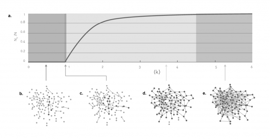
Evolution of a random network. The relative size of the giant component in function of the average degree ‹k› in the Erdős-Rényi model. The figure illustrates the phase tranisition at ‹k› = 1, responsible for the emergence of a giant component with nonzero NG (source)

Apart of the Erdős Model, there are some other methods to generate networks, such as configurational models, where the number of edges are pre-configured on initialization, so the generated mesh will consist of vertices with pre configured edge connectedness. Qualitative models are starting from an organized network where local components are connected, and the edges are reconfigured through randomisation to connect distant areas of the network.

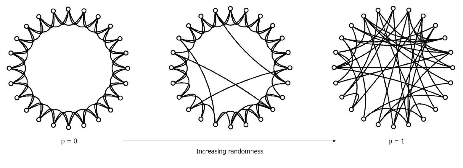
Watz-Strogatz Graph Generation Model (source)

The code I wrote is about to visualize a simple force directed graph with vertices and edges, where the graph can be built from a list of parameters stored in a csv file, or the components of the graphs can be added to the system individually, with different connection configurations. Later on, connectedness, betweenness, the presence of motives are planned to be visualized with the code. A vertex's edge number is defining the size of the vertex at the moment.

Generating graph: each new node is connected randomly to a previous existing node. No clusters and triangles arise.


Generating graph: each new node is connected to all existing nodes. Heavy clusterization.


Generating graph: each new node can be connected to any existing node with a probability of 0.1. Some clusters arise, there are also vertices that have no edges.


Generating graph: each new node is connected randomly to one of the first three elements. The result is a heavily centralized network.
 

Random notes from the workshop:
There are basically 16 different motifs can be found in directed graphs. Large scale graph characteristics can be visualized by their motif frequency distributions respectively. Interesting example is the "triangle closure" that can be found in social networks: motifs start forming closed triangles by time.

Usually network connectedness is high within local areas and low on the global scale.

The "network approach" is more sensitive to the cleanliness of data compared to other analytic methods.

(Network based) Data analysis usually consists of the following steps:

Complex System -> Data -> Network -> Mathematical Quantities -> Representational Qualities -> Conclusion

Mathematical quantities can be described by computation, whereas representational qualities are thoughtfully interpreted aspects that can be used for visualization.