IO

ML Techniques for Realtime Interaction

This post is a non comprehensive overview of some key techniques used for Machine Learning, from a perspective that is focusing on realtime interaction and creative process, covering techniques from traditional supervised learning to reinforced learning. Think of it as a list of notes to the self (or a cheatsheat) that will help define my following weeks of research.

Basically, Machine Learning is divided into three main categories: supervised learning, unsupervised learning and a combination of these (reinforced learning). Supervised learning is useful in cases where a property (label) is available for a certain dataset (training set), but is missing and needs to be predicted for other instances. It requires at least two data sets, a training set which consists of inputs with the expected output, and a testing set which consists of inputs without the expected output. Both of these data sets must consist of labelled data i.e. data patterns for which the target is known upfront. I am using supervised techniques for my gesture recognizer with leap motion, but I also use supervised learning for my audio classification and semantic content visualization experiments. Unsupervised learning is useful in cases where the challenge is to discover implicit relationships in a given unlabeled dataset (items are not pre-assigned). This works best if you have plenty of data (usually organized into datasets). Unsupervised strategies are typically used to discover hidden structures (such as hidden Markov chains) in unlabeled data. I was using unsupervised learning as dimensionaly reduction (based on t-SNE algorithm) when trying to find meaningful relationship in collections. Reinforcement learning falls between these 2 extremes — there is some form of feedback available for each predictive step or action, but no precise label or error message.

Classification
Classification is a general process related to categorization, the process in which ideas and objects are recognized, differentiated, and understood. The examples below illustrate the visual results of different supervised learning algorithms that are trained on the same data. These algorithms are trying to find the decision boundaries of three different classes which are indicated with three different shades of gray color. The edges are highlighted in each image in order to get a grasp on how the algorithm defines its decision boundaries. The images are generated with the algorithms from Nick Gillian's Gesture Recognition Toolkit

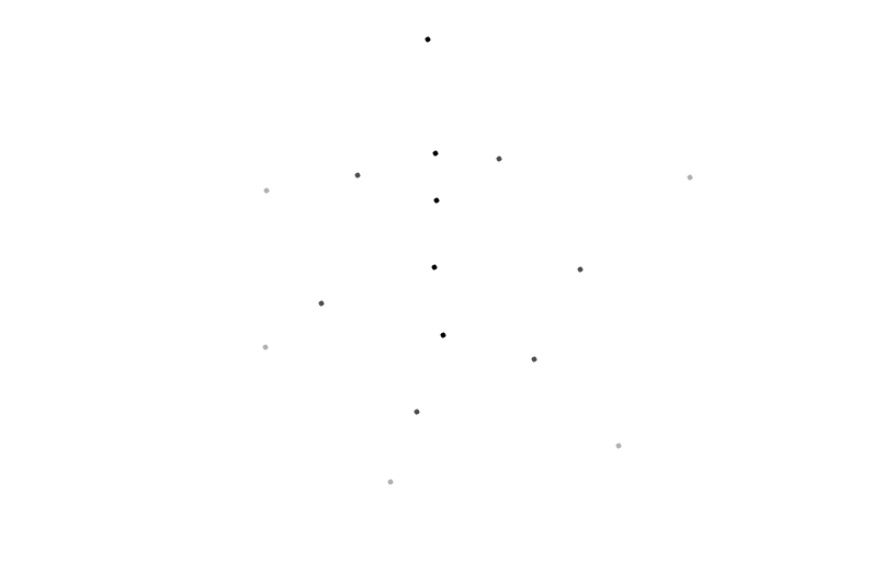
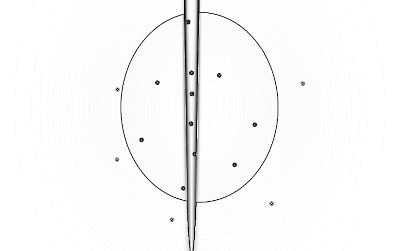
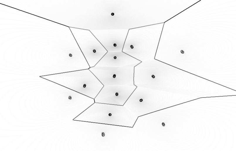
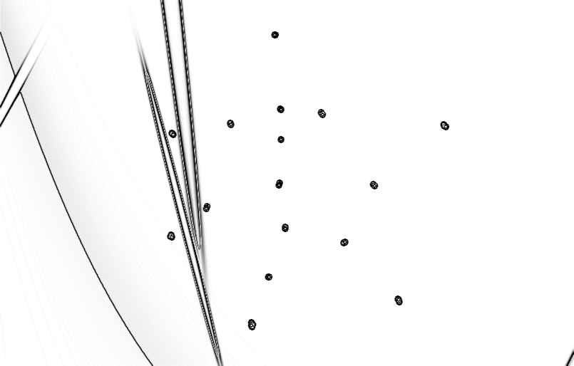
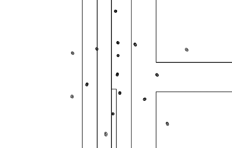
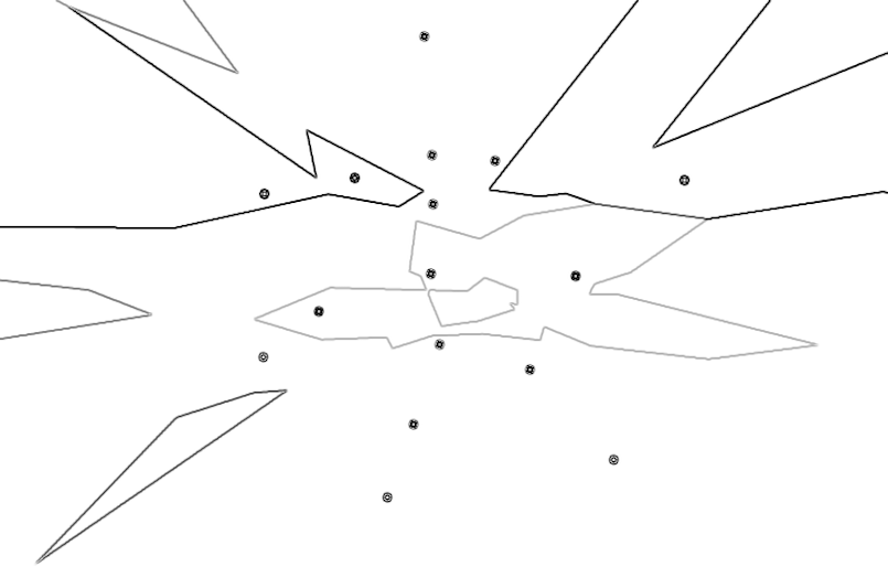
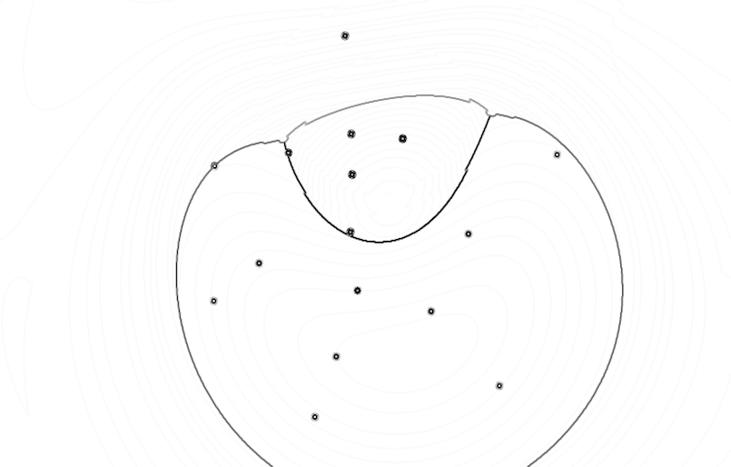
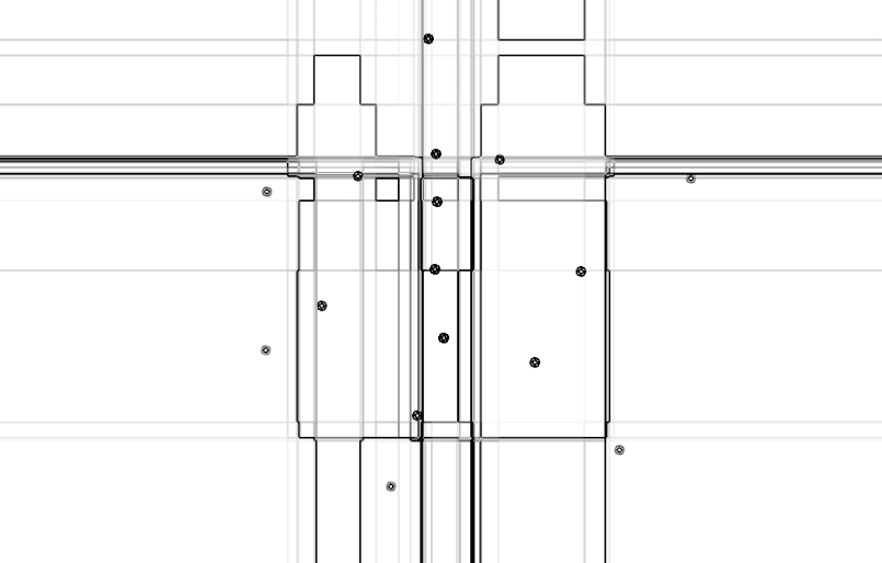
1. Original training examples, 2. Naive Bayes, 3. Mindist, 4. Gaussian Mixture Model, 5. Decision Tree, 6. k-Nearest Neighbor, 7. Support Vector Machine, 8. Adaboost
(right-click to view in larger size)

I made a comparision of those algorithms on labeled semantic audio in another post, to see how they work in a more real-world scenario. Streamlined, simple description of these techniques can be read in the 2015 NIME paper of ml-lib (a software library implementing Gesture Recognition Toolkit within Pure Data / Max):

Adaboost
AdaBoost (Adaptive Boosting) is a powerful classifier that works well on both basic and more complex recognition problems. AdaBoost works by creating a highly accurate classifier by combining many relatively weak and inaccurate classifiers. AdaBoost therefore acts as a meta algorithm, which allows you to use it as a wrapper for other classifiers.’

Decision Tree
‘Decision Trees are conceptually simple classifiers that work well on even complex classification tasks. Decision Trees partition the feature space into a set of rectangular regions, classifying a new datum by finding which region it belongs to.’ ‘A decision tree is a flowchart-like structure in which each internal node represents a test on an attribute (e.g. whether a coin flip comes up heads or tails), each branch represents the outcome of the test and each leaf node represents a class label (decision taken after computing all attributes). The paths from root to leaf represents classification rules.’

Gaussian Mixture Model
The Gaussian Mixture Model Classifier (GMM) is basic but useful supervised learning classification algorithm that can be used to classify a wide variety of N-dimensional signals.’

k-Nearest Neighbor
‘The K-Nearest Neighbor (KNN) Classifier is a simple classifier that works well on basic recognition problems, however it can be slow for real-time prediction if there are a large number of training examples and is not robust to noisy data. In pattern recognition, the k-Nearest Neighbors algorithm (or k-NN for short) is a non-parametric method used for classification and regression. In both cases, the input consists of the k closest training examples in the feature space.’

Support Vector Machine
‘In machine learning, support vector machines (SVMs, also support vector networks) are supervised learning models with associated learning algorithms that analyze data and recognize patterns, used for classification and regression analysis. Given a set of training examples, each marked as belonging to one of two categories, an SVM training algorithm builds a model that assigns new examples into one category or the other, making it a non-probabilistic binary linear classifier. An SVM model is a representation of the examples as points in space, mapped so that the examples of the separate categories are divided by a clear gap that is as wide as possible. New examples are then mapped into that same space and predicted to belong to a category based on which side of the gap they fall on.’ Also, see previous post.

Regression
Regression is another ML method that can be made with supervised learning. We can think of linear regression as the task of fitting a straight line through a set of points. There are multiple possible strategies to do this, in the case of linear regression, we can draw a line, and then for each of the data points, measure the vertical distance between the point and the line, and add these up; the fitted line would be the one where this sum of distances is as small as possible. Logistic regression is similar, but instead of a line it is using  a logistic function, which is the cumulative logistic distribution. Regression can be used for such cases like predictions, where probabilities are more important to know than finding out labels of data.

Unsupervised Learning
Unsupervised learning is very effective in clustering algorithms: Clustering is the task of grouping a set of objects such that objects in the same group (cluster) are more similar to each other than to those in other groups. The t-distributed stochastic neighbor embedding (t-SNE) is a nonlinear dimensionality reduction technique that is particularly well-suited for embedding high-dimensional data into a space of two or three dimensions, which can then be visualized in a scatter plot. Specifically, it models each high-dimensional object by a two- or three-dimensional point in such a way that similar objects are modeled by nearby points and dissimilar objects are modeled by distant points. The t-SNE algorithm comprises two main stages. First, t-SNE constructs a probability distribution over pairs of high-dimensional objects in such a way that similar objects have a high probability of being picked, whilst dissimilar points have an extremely small probability of being picked. Second, t-SNE defines a similar probability distribution over the points in the low-dimensional map, and it minimizes the divergence between the two distributions with respect to the locations of the points in the map. 

Neural Networks
A neural network is a “connectionist” computational system. Everyday computational systems we write are procedural; a program starts at the first line of code, executes it, and goes on to the next, following instructions in a linear fashion. A true neural network does not follow a linear path. Rather, information is processed collectively, in parallel throughout a network of nodes (the nodes, in this case, being neurons). 

The most common learning algorithm for neural networks is the backpropagation algorithm which uses stochastic gradient descent. Backpropagation consists of two steps: The feedforward pass -  the training data set is passed through the network and the output from the neural network is recorded and the error of the network is calculated, and Backward propagation - the error signal is passed back through the network and the weights of the neural network are optimized using gradient descent.

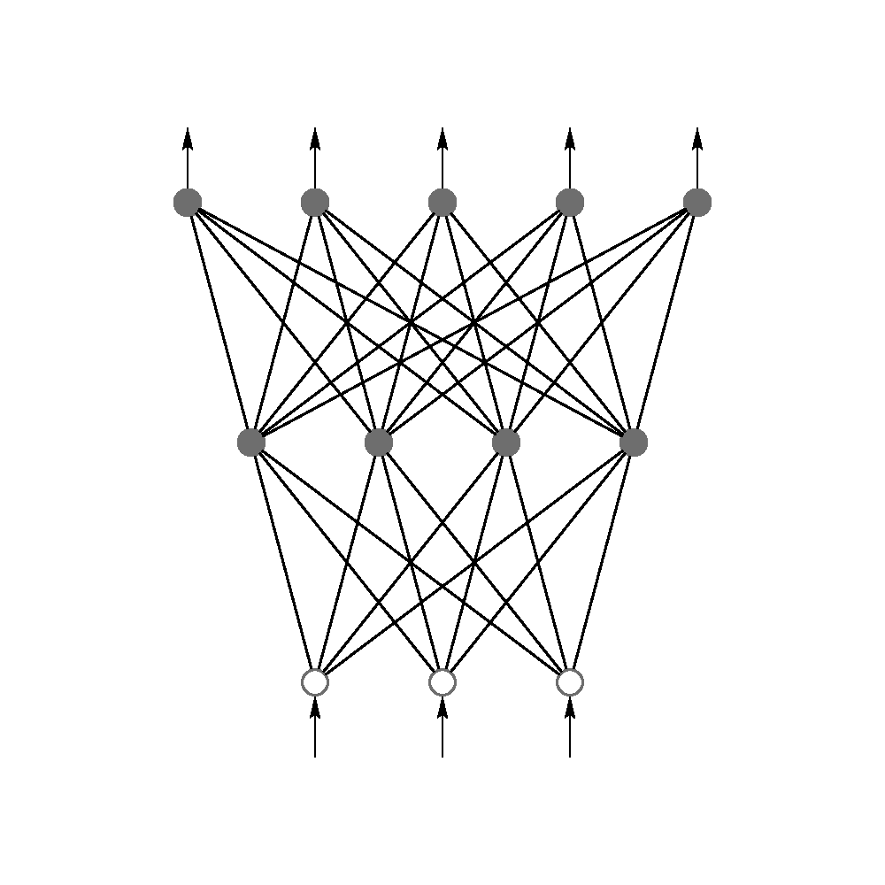
A 2-layered feedforward neural network, from top to bottom:
an output layer with 5 units, a hidden layer with 4 units, respectively.
The network has 3 input units source

FeedForward Neural Networks (FFNN)
The feedforward neural network was the first and arguably most simple type of artificial neural network devised. In this network the information moves in only one direction—forward: From the input nodes data goes through the hidden nodes (if any) and to the output nodes. There are no cycles or loops in the network. Feedforward networks can be constructed from different types of units, the simplest example being the perceptron. Continuous neurons, frequently with sigmoidal activation, are used in the context of backpropagation of error.

Convolutional neural networks (CNN, or ConvNet)
CNN is a type of feed-forward artificial neural network in which the connectivity pattern between its neurons is inspired by the organization of the animal visual cortex. Individual cortical neurons respond to stimuli in a restricted region of space known as the receptive field. The receptive fields of different neurons partially overlap such that they tile the visual field. The response of an individual neuron to stimuli within its receptive field can be approximated mathematically by a convolution operation. Convolutional networks were inspired by biological processes and are variations of multilayer perceptrons designed to use minimal amounts of preprocessing. They have wide applications in image and video recognition, recommender systems and natural language processing.

Recurrent neural networks (RNN) 
These are FFNNs with a time twist: they are not stateless; they have connections between passes, connections through time. Neurons are fed information not just from the previous layer but also from themselves from the previous pass. This means that the order in which you feed the input and train the network matters. One big problem with RNNs is the vanishing (or exploding) gradient problem where, depending on the activation functions used, information rapidly gets lost over time, just like very deep FFNNs lose information in depth. Intuitively this wouldn’t be much of a problem because these are just weights and not neuron states, but the weights through time is actually where the information from the past is stored; if the weight reaches a value of 0 or 1 000 000, the previous state won’t be very informative. 

Long / short term memory (LSTM) networks
LSTMS try to combat the vanishing / exploding gradient problem by introducing gates and an explicitly defined memory cell. These are inspired mostly by circuitry, not so much biology. Each neuron has a memory cell and three gates: input, output and forget. The function of these gates is to safeguard the information by stopping or allowing the flow of it. The input gate determines how much of the information from the previous layer gets stored in the cell. The output layer takes the job on the other end and determines how much of the next layer gets to know about the state of this cell. 

If you'd like to find out more about different beasts of neural networks, visit Van Veen's Zoo, where there are much more specific and detailed information on the genres incarnations and underlying structures of them.

Reinforcement learning 
RL is an area of machine learning inspired by behaviorist psychology, concerned with how software agents ought to take actions in an environment so as to maximize some notion of cumulative reward. The problem, due to its generality, is studied in many other disciplines, such as game theory, control theory, operations research, information theory, simulation-based optimization, multi-agent systems, swarm intelligence, statistics, and genetic algorithms. In the operations research and control literature, the field where reinforcement learning methods are studied is called approximate dynamic programming. The technique is similar to supervised learning, but instead of training them on correct labels, they have to figure out what features to learn.

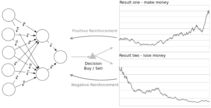
A Neural network can be reinforced both negatively
and positively source

Reinforcement learning strategies consist of three components. A policy which specifies how the neural network will make decisions e.g. using technical and fundamental indicators. A reward function which distinguishes good from bad e.g. making vs. losing money. And a value function which specifies the long term goal. There is a really inspiring writeup by A. Karpathy on how a network can learn playing Pong based on raw pixel data. It also shows differences between the creative way of human learning and the dumb, statistical way of machines.